Introduction to mccount • mccount

Introduction

When studying diseases and medical interventions, patients often experience events that can occur multiple times (e.g., hospitalizations, infections, or tumor recurrences). Traditional survival analysis methods typically focus on time to the first event, potentially missing important information about the total disease burden.

Many patients experience events that can occur multiple times—like hospital readmissions, infections, or tumor recurrences. Traditional survival analysis is only concerned with the first event and does not account for competing risks like death. Alternatively, the mean cumulative count (MCC) provides a more complete picture by estimating the expected number of events per person by a given time, properly accounting for:

Multiple occurrences of the same event (recurrent events)
Events that prevent future occurrences (competing risks like death)
Incomplete follow-up (censoring)

library(mccount)
library(dplyr)
library(survival)

Clinical Example: Bladder Cancer Recurrences

We’ll use the survival::bladder1 dataset from the survival package, which contains data on bladder cancer recurrences from a randomized trial comparing three treatments: placebo, pyridoxine, and thiotepa.

The bladder1 dataset contains 118 patients followed for tumor recurrences. The key variables are:

id: Patient identifier
stop: Time of event or censoring
status: Event type (0 = censored, 1 = recurrence, 2 = death from bladder disease, 3 = death from other cause)
treatment: Treatment group (placebo, pyridoxine, or thiotepa)

Data Preparation

For MCC analysis, we need to ensure our competing event variable has the proper coding:

0 = censoring
1 = event of interest (recurrence)
2 = competing event (death from any cause)

# Prepare data for MCC analysis
bladder_mcc <- bladder1 |>
  # Combine death causes into a single competing event indicator
  mutate(status = if_else(status >= 2, 2, status))

Basic MCC Analysis

Let’s calculate the MCC of bladder cancer recurrences for the entire cohort:

# Calculate MCC using the Dong-Yasui equation method
mcc_overall <- mcc(
  data = bladder_mcc,
  id_var = "id",
  time_var = "stop",
  cause_var = "status"
)
#> Warning: Found 13 participants where last observation is an event of interest
#> (`cause_var` = 1)
#> First 5 IDs: 13, 15, 16, 19, 24
#> Total affected: 13 participants
#> ℹ `mcc()` assumes these participants are censored at their final `time_var`
#> ℹ If participants were actually censored or experienced competing risks after
#>   their last event, add those observations to ensure correct estimates

Notice that mcc() will warn the user if there are participants whose data end do not explicitly have a censoring event (0) of competing event (2) on their final row. The function provides this warning to ensure the user is aware of this and also aware of how this is implicitly interpreted by the package. The function also lets the user know that the MCC estimate will be incorrect if the mccount’s implicit assumption is incorrect.

Available Estimators

The mcc() function can be used to calculate the MCC using either the Dong-Yasui estimator (method = "equation", the default) or the sum of cumulative incidence estimator (method = "sci"). See vignette("choosing-between-methods") and ?mcc for more details.

Understanding the Output

Just calling the mcc object we’ve created will print the method used, a preview of the MCC estimates at each time point, and the exact mcc() call used to generate the output:

mcc_overall
#> 
#> ── Mean Cumulative Count Results ───────────────────────────────────────────────
#> ℹ Method: Dong-Yasui Equation Method
#> 
#> ── MCC Estimates ──
#> 
#> # A tibble: 6 × 2
#>    time    mcc
#>   <int>  <dbl>
#> 1     0 0     
#> 2     1 0.0256
#> 3     2 0.112 
#> 4     3 0.241 
#> 5     4 0.276 
#> 6     5 0.320
#> # ... with 45 more rows
#> ── Call ──
#> 
#> mcc(data = bladder_mcc, id_var = "id", time_var = "stop", cause_var = "status")

The package also includes an S3 method for the summary() function that will output more useful details:

# Get summary statistics
summary(mcc_overall)
#> 
#> ── Summary of Mean Cumulative Count Results ────────────────────────────────────
#> ℹ Method: Dong-Yasui Equation Method
#> ℹ Total participants: 118
#> 
#> ── Summary Statistics ──
#> 
#> Observation period: [0, 64]
#> Time to MCC = 1.0: 22
#> Time to maximum MCC: 53
#> MCC at end of follow-up: 2.2672
#> 
#> ── Event Count Composition
#> Events of interest: 189
#> Competing risk events: 29
#> Censoring events: 76

We can also extract the MCC estimate at the end of study follow-up using mcc_final_values(mcc_overall) and/or extract the MCC values at specific time points (not only the MCC at the end of follow-up). For example:

# Extract key timepoints
key_times <- c(6, 12, 24, 36, 48, 60)  # months
mcc_at_times <- mcc_overall$mcc_table |>
  filter(time %in% key_times) |>
  mutate(
    years = time / 12,
    mcc = cards::round5(mcc, 3)
  ) |>
  select(years, time, mcc)

mcc_at_times
#> # A tibble: 6 × 3
#>   years  time   mcc
#>   <dbl> <int> <dbl>
#> 1   0.5     6 0.391
#> 2   1      12 0.622
#> 3   2      24 1.16 
#> 4   3      36 1.64 
#> 5   4      48 2.03 
#> 6   5      60 2.27

Visualization

mccount provides flexible plotting capabilities that can be combined with ggplot2 functions/syntax:

# Basic plot
plot(mcc_overall) +
  labs(
    title = "Bladder Cancer Recurrence Burden",
    subtitle = "Mean cumulative count over time",
    x = "Time (Months)"
  ) +
  scale_x_continuous(
    breaks = c(seq(
      0, max(mcc_overall$mcc_table$time), 
      by = 12
      )
    )) +
    geom_line_mcc(mcc_overall)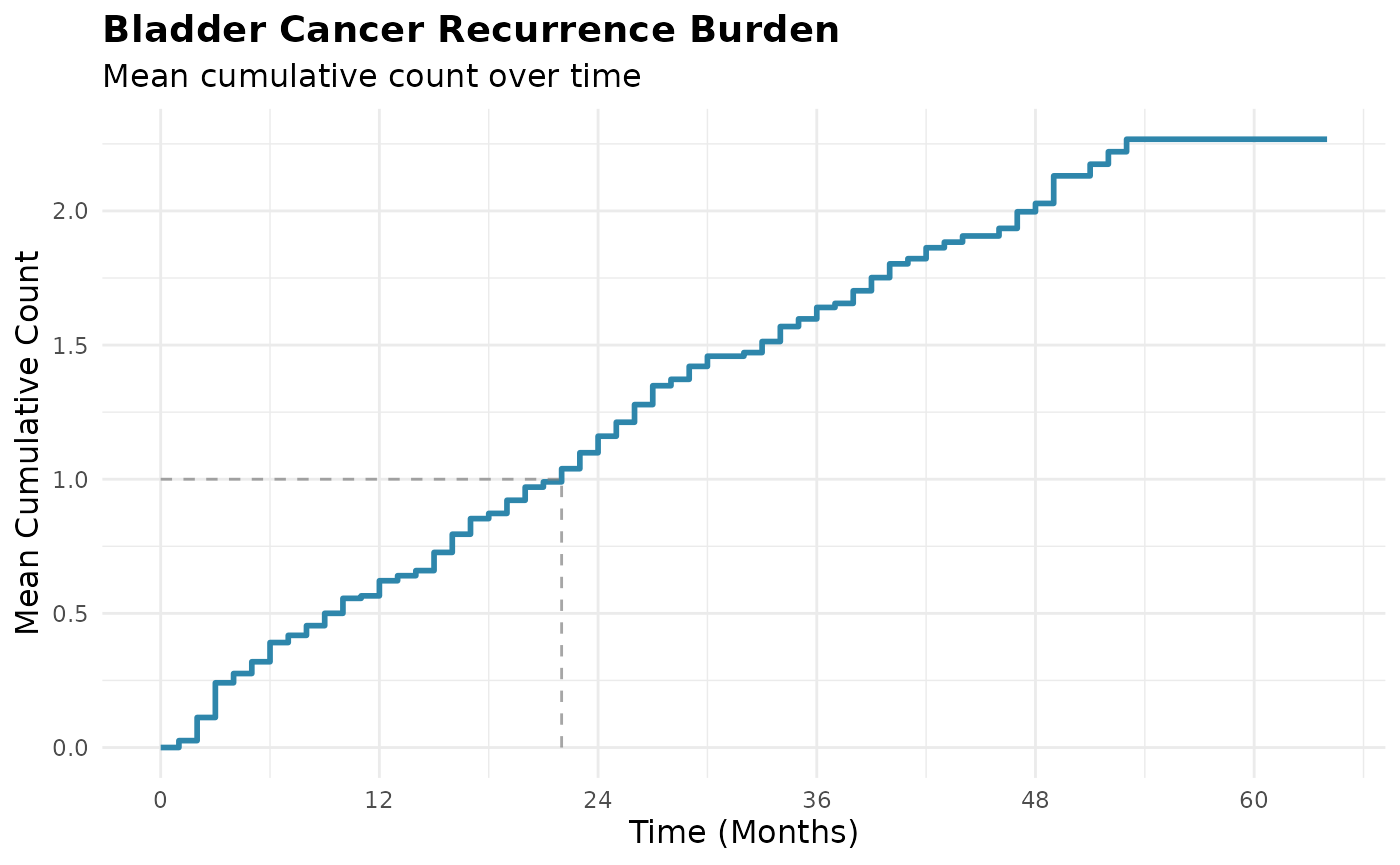

The step function shows how the expected number of bladder cancer recurrences accumulates over the entire study follow-up period.

MCC Interpretation

The estimated MCC can be interpreted as the number of events per person we expect among individuals who have not experienced a competing risk event by a given time. Looking at the print out from summary(mcc_overall), the MCC at the end of follow-up is 2.27 - on average, each bladder cancer survivor experiences 2.27 recurrences by 64 months.

In a population of 100 similar patients, we expect approximately 2.27 * 100 = 227 total recurrences by 64 months. This accounts for the fact that some patients die and cannot experience further recurrences.

Dong, et al.¹ provide additional guidance for interpreting the MCC (emphasis added):

Note that MCC is a marginal measure (as opposed to a conditional measure) of disease burden, similar to [cumulative incidence], and its interpretation is not conditional on survival free of competing risk events. Also, MCC does not assume independence between the event of interest and the competing-risk event.

Stratifying by Treatment Groups

It’s common that we may want to estimate the MCC stratified by a specific characteristic, like "treatment" group. mcc() provides a simple by argument to assist with this:

# Calculate MCC by treatment group
mcc_by_treatment <- mcc(
  data = bladder_mcc,
  id_var = "id",
  time_var = "stop",
  cause_var = "status",
  by = "treatment",
  method = "equation"
)
#> Warning: Found 7 participants where last observation is an event of interest
#> (`cause_var` = 1)
#> First 5 IDs: 13, 15, 16, 19, 24
#> Total affected: 7 participants
#> ℹ `mcc()` assumes these participants are censored at their final `time_var`
#> ℹ If participants were actually censored or experienced competing risks after
#>   their last event, add those observations to ensure correct estimates
#> Warning: Found 4 participants where last observation is an event of interest
#> (`cause_var` = 1)
#> ! ID: 51, 64, 67, 70
#> ℹ `mcc()` assumes these participants are censored at their final `time_var`
#> ℹ If participants were actually censored or experienced competing risks after
#>   their last event, add those observations to ensure correct estimates
#> Warning: Found 2 participants where last observation is an event of interest
#> (`cause_var` = 1)
#> ! ID: 83, 104
#> ℹ `mcc()` assumes these participants are censored at their final `time_var`
#> ℹ If participants were actually censored or experienced competing risks after
#>   their last event, add those observations to ensure correct estimates

# Summary by group
summary(mcc_by_treatment)
#> 
#> ── Summary of Mean Cumulative Count Results ────────────────────────────────────
#> ℹ Method: Dong-Yasui Equation Method
#> ℹ Total participants: 118
#> ℹ Overall observation period: [0, 64]
#> 
#> ── Summary by Group (treatment) ──
#> 
#> ── Group: placebo
#> Participants in group: 48
#> Group observation period: [0, 64]
#> Time to MCC = 1.0: 17
#> Time to maximum MCC: 53
#> MCC at end of follow-up: 2.6137
#> Events of interest: 87
#> Competing risk events: 11
#> Censoring events: 30
#> 
#> ── Group: pyridoxine
#> Participants in group: 32
#> Group observation period: [0, 60]
#> Time to MCC = 1.0: 19
#> Time to maximum MCC: 49
#> MCC at end of follow-up: 2.5831
#> Events of interest: 57
#> Competing risk events: 7
#> Censoring events: 21
#> 
#> ── Group: thiotepa
#> Participants in group: 38
#> Group observation period: [0, 59]
#> Time to MCC = 1.0: 27
#> Time to maximum MCC: 47
#> MCC at end of follow-up: 1.5463
#> Events of interest: 45
#> Competing risk events: 11
#> Censoring events: 25

Visualizing Treatment Differences

The other functions in mccount automatically recognize the mcc_grouped S3 class and adjust their behavior accordingly. For example, we can feed mcc_by_treatment into plot(), and it automatically knows to plot an MCC curve by the stratification variable.

# Plot with treatment groups
plot(mcc_by_treatment) +
  labs(
    title = "Bladder Cancer Recurrence Burden by Treatment",
    subtitle = "Mean cumulative count over time",
    x = "Time (Months)",
    color = "Treatment"
  ) +
  scale_x_continuous(
    breaks = seq(
      0, max(mcc_by_treatment$original_data$time), 
      by = 12
      )
    ) +
    geom_line_mcc(mcc_by_treatment)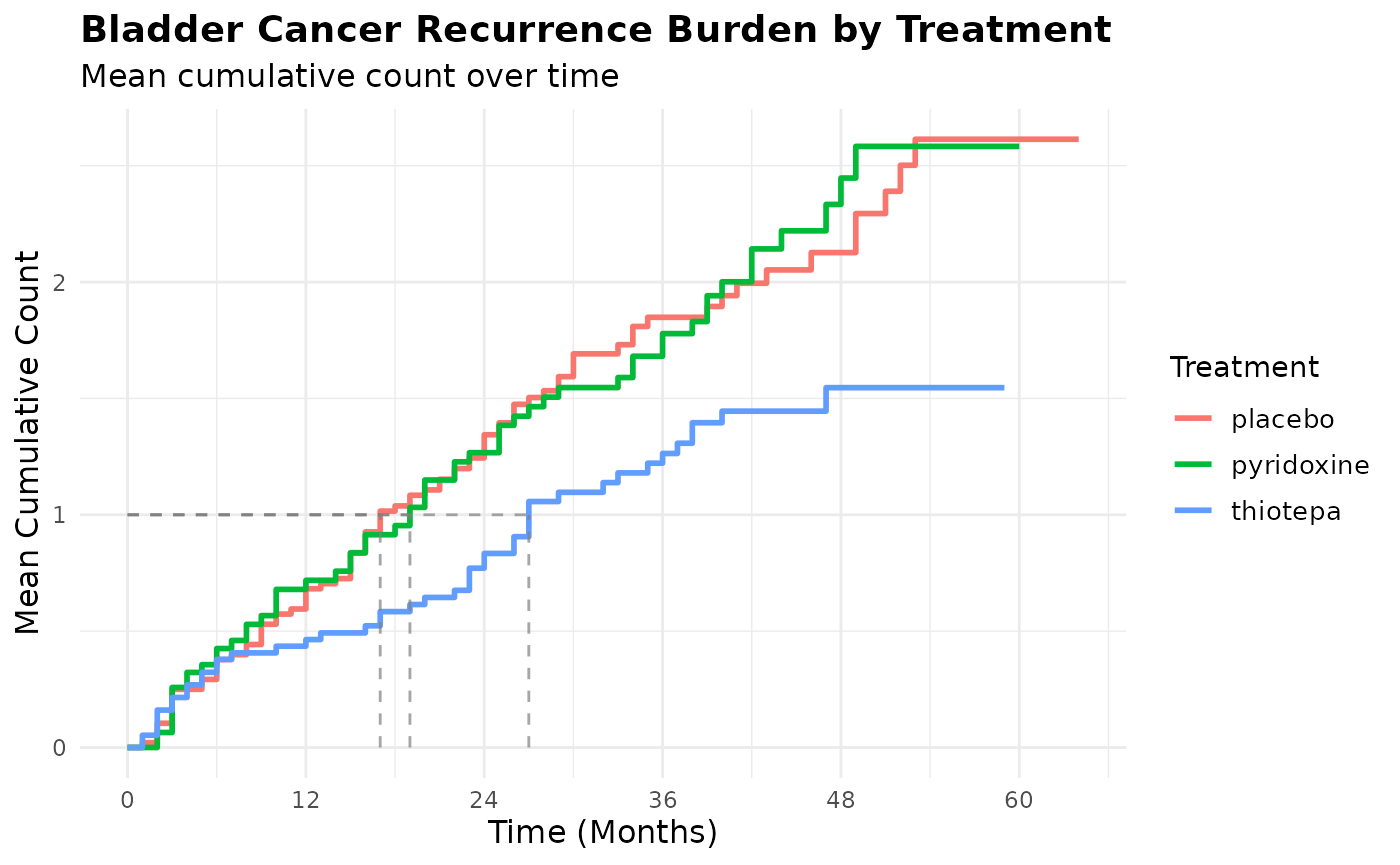

Confidence intervals for the MCC can be generated via bootstrapping.

Weighted MCC Analysis

mccount also allows estimation of weighted MCC in the setting of observational studies that want to account for measured confounding and/or other types of bias via matching or weighting. See the vignette("estimating-mcc-after-matching-or-weighting") for more details.