Plot MCC results — plot.mcc • mccount

Creates plots for Mean Cumulative Count (MCC) results. The plotting method automatically adapts based on the mcc object class and whether the analysis was grouped.

Usage

# S3 method for class 'mcc'
plot(
  x,
  type = c("mcc", "components"),
  groups = NULL,
  conf_int = FALSE,
  colors = NULL,
  title = NULL,
  subtitle = NULL,
  ...
)

Arguments

x

An mcc object

type

Character string specifying plot type:

"mcc" (default): Plot MCC estimates over time
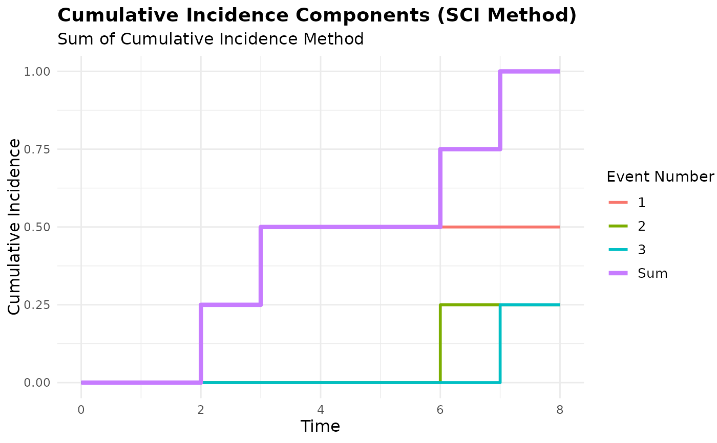
"components": Show individual cumulative incidence components (SCI method only)

groups

Character vector specifying which groups to include in grouped analyses. If NULL (default), all groups are included

conf_int

Logical indicating whether to include confidence intervals if available

colors

Character vector of colors to use for groups. If NULL, uses default colors

title

Character string for plot title. If NULL, generates automatic title

subtitle

Character string for plot subtitle. If NULL, generates automatic subtitle

...

Additional arguments passed to ggplot2 functions

Value

A ggplot2 object

Examples

if (FALSE) { # \dontrun{
# Create sample data
df <- data.frame(
  id = c(1, 2, 3, 4, 4, 4, 5, 5),
  time = c(8, 1, 5, 2, 6, 7, 3, 3),
  cause = c(0, 0, 2, 1, 1, 1, 1, 2),
  group = c("A", "A", "B", "B", "B", "B", "A", "A")
)

# Calculate MCC
mcc_result <- mcc(df, "id", "time", "cause")

# Plot MCC over time
plot(mcc_result)

# SCI method with components plot
mcc_sci <- mcc(df, "id", "time", "cause", method = "sci")
plot(mcc_sci, type = "components")
} # }

# Create sample data
library(dplyr)
df <- data.frame(
  id = c(1, 2, 3, 4, 4, 4, 5, 5),
  time = c(8, 1, 5, 2, 6, 7, 3, 3),
  cause = c(0, 0, 2, 1, 1, 1, 1, 2),
  group = c("A", "A", "B", "B", "B", "B", "A", "A")
) |>
  arrange(id, time)

# Basic MCC plot (ungrouped)
mcc_result <- mcc(df, "id", "time", "cause")
#> Warning: Found 1 participant where last observation is an event of interest (`cause_var`
#> = 1)
#> ! ID: 4
#> ℹ `mcc()` assumes these participants are censored at their final `time_var`
#> ℹ If participants were actually censored or experienced competing risks after
#>   their last event, add those observations to ensure correct estimates
#> ℹ Adjusted time points for events occurring simultaneously for the same subject.
plot(mcc_result)


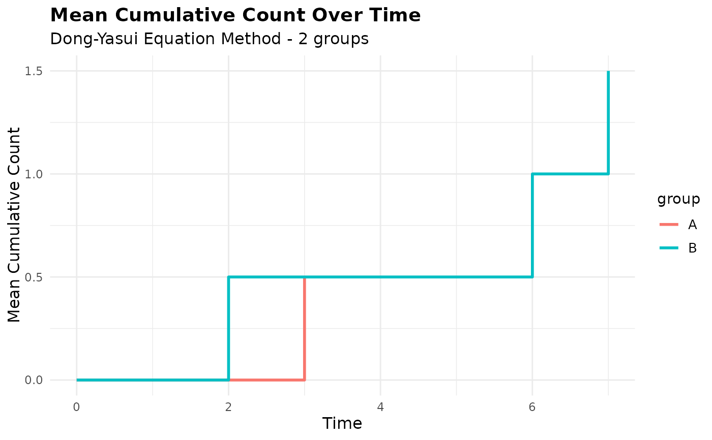
# Grouped analysis with custom colors
mcc_grouped <- mcc(df, "id", "time", "cause", by = "group")
#> ℹ Adjusted time points for events occurring simultaneously for the same subject.
#> Warning: Found 1 participant where last observation is an event of interest (`cause_var`
#> = 1)
#> ! ID: 4
#> ℹ `mcc()` assumes these participants are censored at their final `time_var`
#> ℹ If participants were actually censored or experienced competing risks after
#>   their last event, add those observations to ensure correct estimates
plot(mcc_grouped)


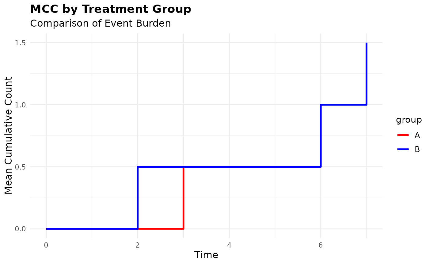
# Customize the grouped plot
plot(mcc_grouped,
     colors = c("red", "blue"),
     title = "MCC by Treatment Group",
     subtitle = "Comparison of Event Burden")


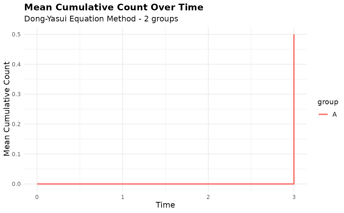
# Plot only specific groups
plot(mcc_grouped, groups = c("A"))


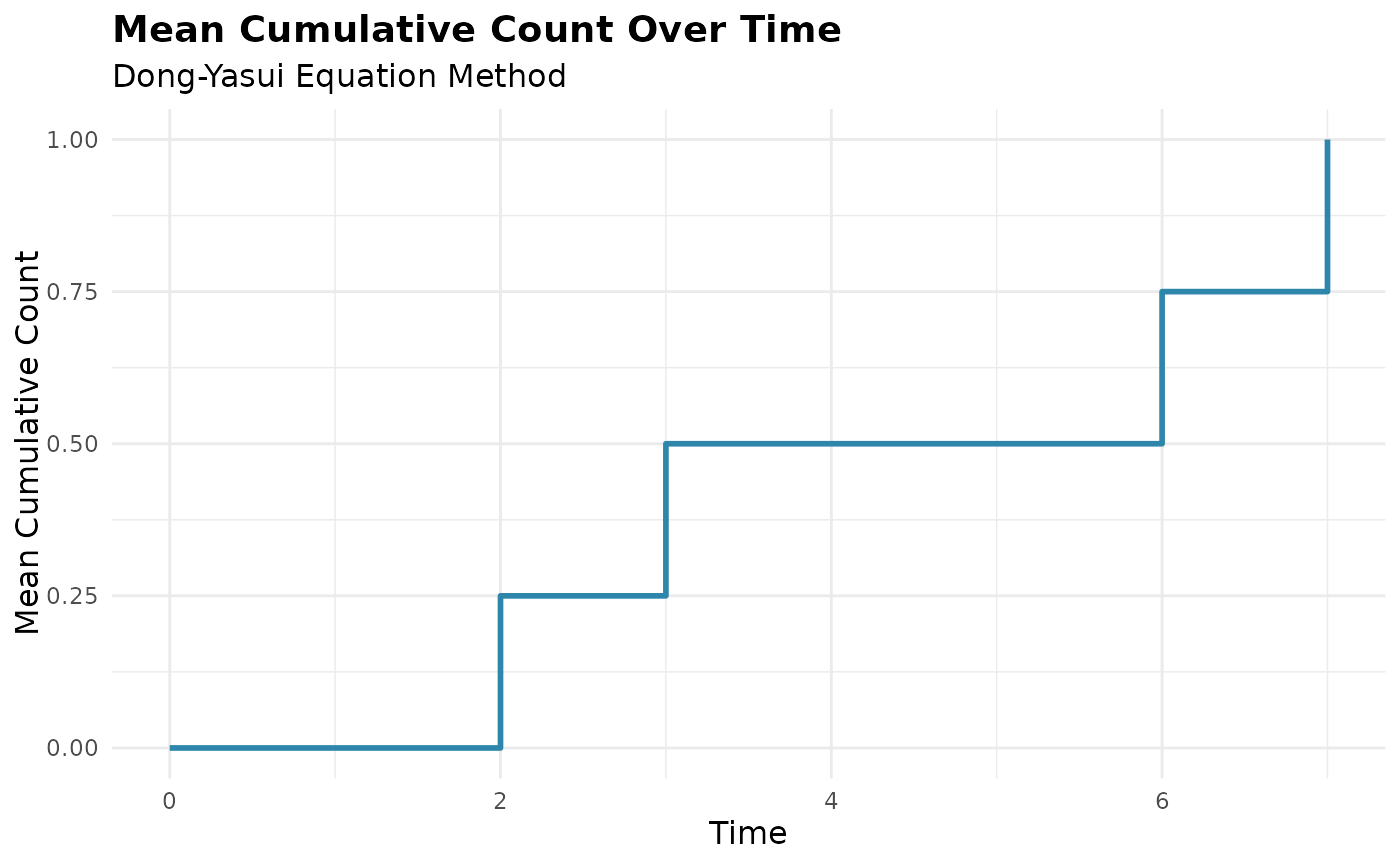
# Compare different methods - equation method only shows MCC
mcc_eq <- mcc(df, "id", "time", "cause", method = "equation")
#> Warning: Found 1 participant where last observation is an event of interest (`cause_var`
#> = 1)
#> ! ID: 4
#> ℹ `mcc()` assumes these participants are censored at their final `time_var`
#> ℹ If participants were actually censored or experienced competing risks after
#>   their last event, add those observations to ensure correct estimates
#> ℹ Adjusted time points for events occurring simultaneously for the same subject.
plot(mcc_eq)


# SCI method can show components of cumulative incidence components
mcc_sci <- mcc(df, "id", "time", "cause", method = "sci")
#> Warning: Found 1 participant where last observation is an event of interest (`cause_var`
#> = 1)
#> ! ID: 4
#> ℹ `mcc()` assumes these participants are censored at their final `time_var`
#> ℹ If participants were actually censored or experienced competing risks after
#>   their last event, add those observations to ensure correct estimates
#> ℹ Adjusted time points for events occurring simultaneously for the same subject.
plot(mcc_sci)  # Shows main MCC plot

plot(mcc_sci, type = "components")  # Shows CI components


# Clean up
rm(df, mcc_result, mcc_grouped, mcc_eq, mcc_sci)